K-Nearest Neighbors (KNN) Algorithm for Supervised Machine Learning

What is a Classification in Machine Learning?
Classification is the process of categorizing a given data set into predefined categories based on their features. For example, you could build a classification model to predict whether a brain tumor is malignant (cancerous) or benign (non cancerous) based on MRI data.
The KNN algorithm can be used for such classification tasks. Let's see how the KNN algorithm works.
How KNN Works
To understand the KNN algorithm we will be working with a BMI dataset provided by Kaggle. Each person is categorized into a BMI category of Extremely Weak, Weak, Normal, Overweight, Obesity and Extreme Obesity based on their gender, height and weight. To make things easier to understand, this dataset has been modified to categorize 22 people into a BMI category based on their height and weight.
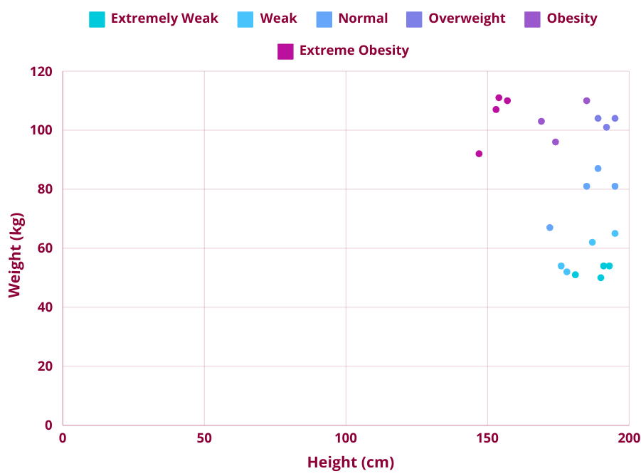
To classify a new data point into a BMI category, the KNN algorithm works as follows:
- Assign a value to K. The K represents the number of neighbors considered in the classification problem. For example, if K is 3 then only 3 nearest neighbors of the new data point will be considered in the classification problem.
- Calculate the distance between the new data point with all of the other existing data points. The distance between the new data point and the nearest neighbors can be calculated using different types of distance metrics such as Euclidean distance, Manhattan distance, Minkowski distance, etc. We will be using Euclidean distance.
- Arrange the calculated distances from Step 2 in ascending order
- Select K data points with the smallest distances. These are the K-Nearest Neighbors of the new data point.
- From the K Neighbors, assign the new data point to the majority class (or a BMI category)
Before we go through a worked example, let's first understand how to calculate the distance between a new data point with all of the other existing data points using the Euclidean distance.
How to find the Euclidean distance
Euclidean distance is the distance between two points (i.e. the length of the line segment between two points). Euclidean distance can be found using Pythagoras theorem. The Euclidean distance formula in a 2D space is:
d = √[(x2 – x1)2 + (y2 – y1)2]
where:
- d is the Euclidean distance
- (x1, y1) is the coordinate of the first point
- (x2, y2) is the coordinate of the second point
Let's go through an example.
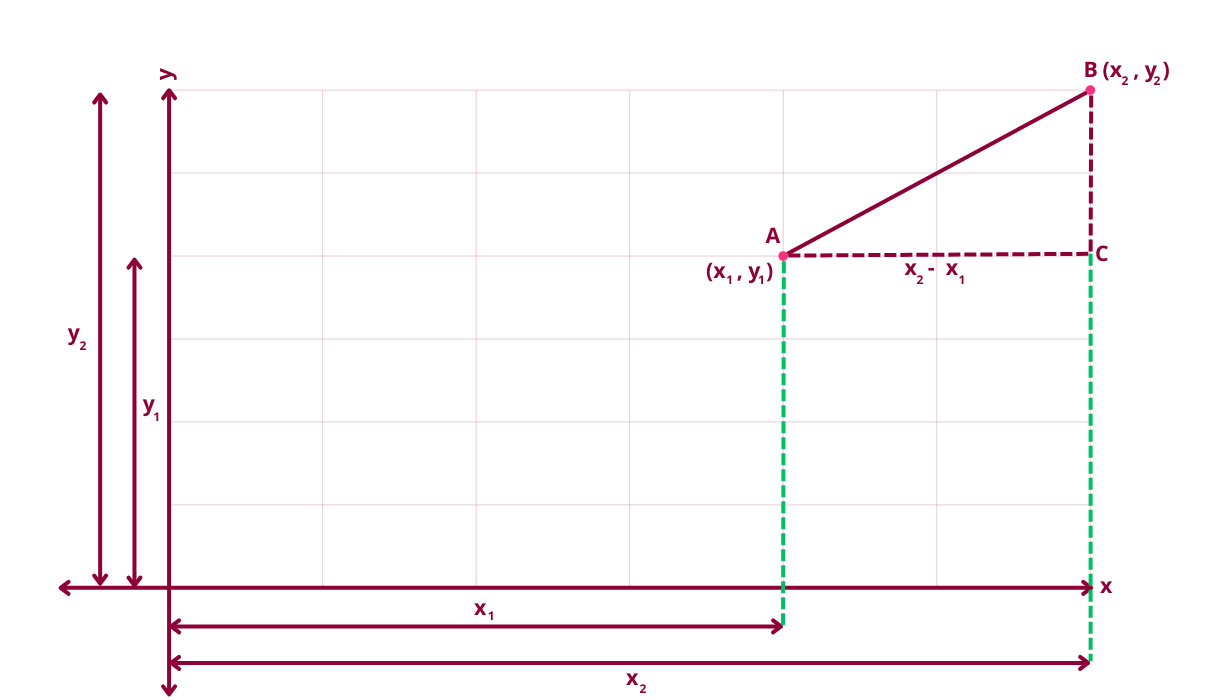
- Let's determine the Euclidean distance between two points A (x1, y1) and B (x2, y2)
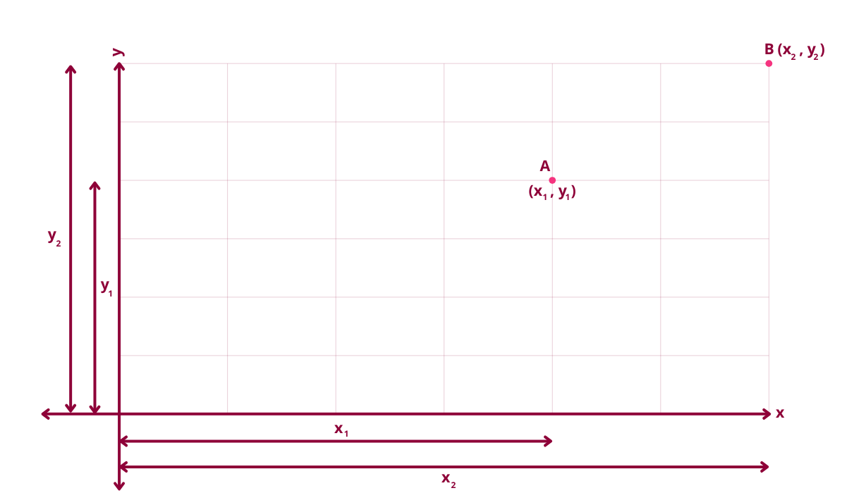
- Join point A with point B using a straight line
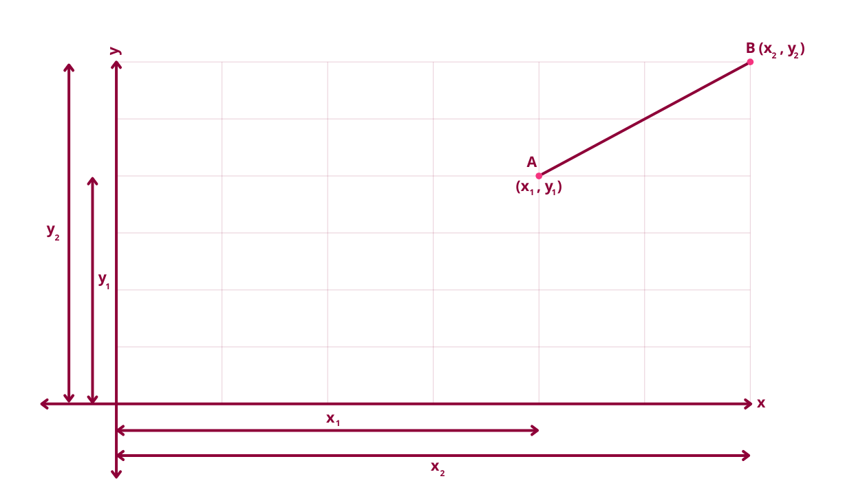
- Create a right-angled triangle. The hypotenuse (the longest side of the right-angled triangle) is AB.
- Draw a horizontal line from point A to C
- Draw a vertical line from point B to C
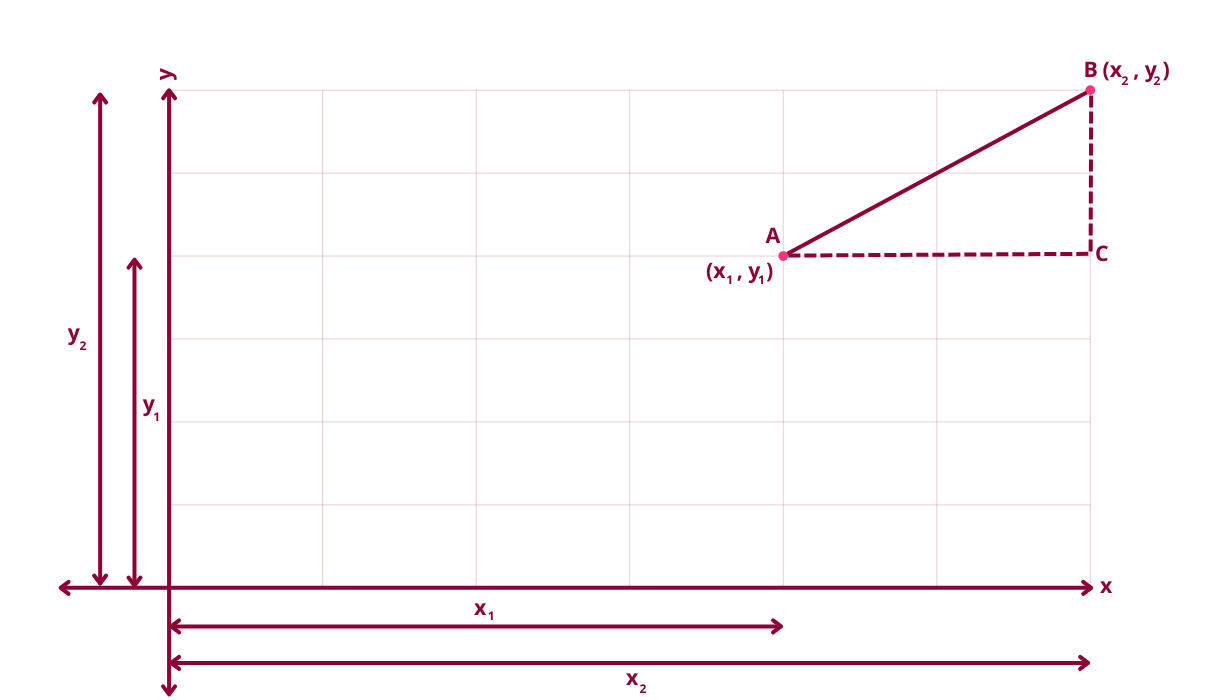
- We can now apply Pythagoras theorem to the triangle ABC to find the distance between A and B. The Pythagoras theorem formula is:
Hypotenuse2 = Base2 + Perpendicular2
If we substitute the values in the formula we get:
AB2 = AC2 + BC2
Let's now calculate the distance between A and C which is simply (x2 – x1)2
Next, let's calculate the distance between B and C which is simply (y2 – y1)2
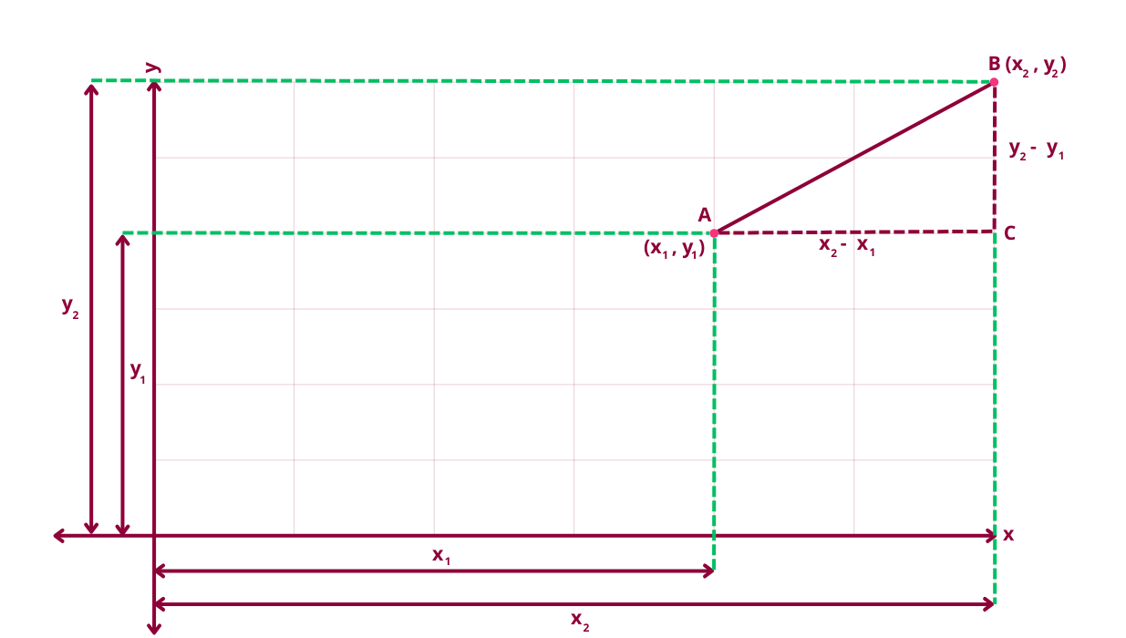
Therefore, d2 = (x2 – x1)2 + (y2 – y1)2
Finally we take the square root on both sides of the equation and the formula for Euclidean distance is derived:
d =√[(x2 – x1)2 + (y2 – y1)2]
A Worked Example of KNN
Let's go through an example of how a new data point is classified using the KNN algorithm. In our data set, we will be classifying person X (the black dot in the diagram below) into a BMI category.
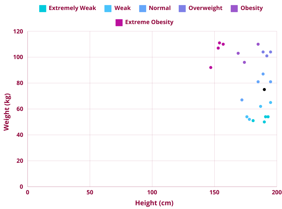
We will be calculating the distance using Euclidean distance and the value of K is 3. To make things easier to work with let's represent the data set as a table. Each person in the table is categorized into a BMI category of Extremely Weak, Weak, Normal, Overweight, Obesity and Extreme Obesity.
| Height | Weight | Group (Classification) |
|---|---|---|
| 193 | 54 | Extremely Weak |
| 181 | 51 | Extremely Weak |
| 191 | 54 | Extremely Weak |
| 190 | 50 | Extremely Weak |
| 187 | 62 | Weak |
| 178 | 52 | Weak |
| 195 | 65 | Weak |
| 176 | 54 | Weak |
| 189 | 87 | Normal |
| 195 | 81 | Normal |
| 172 | 67 | Normal |
| 185 | 81 | Normal |
| 189 | 104 | Overweight |
| 195 | 104 | Overweight |
| 192 | 101 | Overweight |
| 174 | 96 | Obesity |
| 185 | 110 | Obesity |
| 169 | 103 | Obesity |
| 147 | 92 | Extreme Obesity |
| 154 | 111 | Extreme Obesity |
| 153 | 107 | Extreme Obesity |
| 157 | 110 | Extreme Obesity |
The new data point to be classed into a BMI category is:
| Height | Weight | Group (Classification) |
|---|---|---|
| 190 | 75 | ? |
We can now apply the KNN algorithm to class the new data point.
Step 1 - Calculate the Euclidean distance
The new data point (i.e. person to classify into a BMI category) is:
| Height | Weight | Group (Classification) |
|---|---|---|
| 190 | 75 | ? |
The formula for Euclidean distance is:
d =√[(x2 – x1)2 + (y2 – y1)2]
where:
- x2 is the new person's height (in this example it is 190 cm)
- x1 is the existing person's height
- y2 is the new person's weight (in this example it is 75 kg)
- y1 is the existing person's weight
Calculating the Euclidean distance between the new data point and all of the existing data points:
| Height | Weight | Group (Classification) | Euclidean Distance |
|---|---|---|---|
| 193 | 54 | Extremely Weak | √[(190 – 193)2 + (75 – 54)2 ] = 21.21 |
| 181 | 51 | Extremely Weak | √[(190 – 181)2 + (75 – 51)2 ] = 25.63 |
| 191 | 54 | Extremely Weak | √[(190 – 191)2 + (75 – 54)2 ] = 21.02 |
| 190 | 50 | Extremely Weak | √[(190 – 190)2 + (75 – 50)2 ] = 25 |
| 187 | 62 | Weak | √[(190 – 187)2 + (75 – 62)2 ] = 13.34 |
| 178 | 52 | Weak | √[(190 – 178)2 + (75 – 52)2 ] = 25.94 |
| 195 | 65 | Weak | √[(190 – 195)2 + (75 – 65)2 ] = 11.18 |
| 176 | 54 | Weak | √[(190 – 176)2 + (75 – 54)2 ] = 25.23 |
| 189 | 87 | Normal | √[(190 – 189)2 + (75 – 87)2 ] = 12.04 |
| 195 | 81 | Normal | √[(190 – 195)2 + (75 – 81)2 ] = 7.81 |
| 172 | 67 | Normal | √[(190 – 172)2 + (75 – 67)2 ] = 19.69 |
| 185 | 81 | Normal | √[(190 – 185)2 + (75 – 81)2 ] = 7.81 |
| 189 | 104 | Overweight | √[(190 – 189)2 + (75 – 104)2 ] = 29.01 |
| 195 | 104 | Overweight | √[(190 – 195)2 + (75 – 104)2 ] = 29.42 |
| 192 | 101 | Overweight | √[(190 – 192)2 + (75 – 101)2 ] = 26.07 |
| 174 | 96 | Obesity | √[(190 – 174)2 + (75 – 96)2 ] = 26.40 |
| 185 | 110 | Obesity | √[(190 – 185)2 + (75 – 110)2 ] = 35.35 |
| 169 | 103 | Obesity | √[(190 – 169)2 + (75 – 103)2 ] = 35 |
| 147 | 92 | Extreme Obesity | √[(190 – 147)2 + (75 – 92)2 ] = 46.23 |
| 154 | 111 | Extreme Obesity | √[(190 – 154)2 + (75 – 111)2 ] = 50.91 |
| 153 | 107 | Extreme Obesity | √[(190 – 153)2 + (75 – 107)2 ] = 48.91 |
| 157 | 110 | Extreme Obesity | √[(190 – 157)2 + (75 – 110)2 ] = 48.10 |
Step 2 - Arrange Distances in Ascending Order
Rearranging the distances in ascending order:
| Height | Weight | Group (Classification) | Euclidean Distance |
|---|---|---|---|
| 195 | 81 | Normal | 7.81 |
| 185 | 81 | Normal | 7.81 |
| 195 | 65 | Weak | 11.18 |
| 189 | 87 | Normal | 12.04 |
| 187 | 62 | Weak | 13.34 |
| 172 | 67 | Normal | 19.69 |
| 191 | 54 | Extremely Weak | 21.02 |
| 193 | 54 | Extremely Weak | 21.21 |
| 190 | 50 | Extremely Weak | 25 |
| 176 | 54 | Weak | 25.23 |
| 181 | 51 | Extremely Weak | 25.63 |
| 178 | 52 | Weak | 25.94 |
| 192 | 101 | Overweight | 26.07 |
| 174 | 96 | Obesity | 26.40 |
| 189 | 104 | Overweight | 29.01 |
| 195 | 104 | Overweight | 29.42 |
| 169 | 103 | Obesity | 35 |
| 185 | 110 | Obesity | 35.35 |
| 147 | 92 | Extreme Obesity | 46.23 |
| 157 | 110 | Extreme Obesity | 48.10 |
| 153 | 107 | Extreme Obesity | 48.91 |
| 154 | 111 | Extreme Obesity | 50.91 |
Step 3 - Select K-Nearest Neighbors
Since we defined the K value as 3, we will select the top 3 entries from the table:
| Height | Weight | Group (Classification) | Euclidean Distance |
|---|---|---|---|
| 195 | 81 | Normal | 7.81 |
| 185 | 81 | Normal | 7.81 |
| 195 | 65 | Weak | 11.18 |
Step 4 - Assign New Data Point to Majority Class
From the K Neighbors, the majority class is Normal. We can therefore classify the new data point or the new person into a BMI category of Normal. The updated table:
| Height | Weight | Group (Classification) |
|---|---|---|
| 195 | 81 | Normal |
| 185 | 81 | Normal |
| 195 | 65 | Weak |
| 189 | 87 | Normal |
| 187 | 62 | Weak |
| 172 | 67 | Normal |
| 191 | 54 | Extremely Weak |
| 193 | 54 | Extremely Weak |
| 190 | 50 | Extremely Weak |
| 176 | 54 | Weak |
| 181 | 51 | Extremely Weak |
| 178 | 52 | Weak |
| 192 | 101 | Overweight |
| 174 | 96 | Obesity |
| 189 | 104 | Overweight |
| 195 | 104 | Overweight |
| 169 | 103 | Obesity |
| 185 | 110 | Obesity |
| 147 | 92 | Extreme Obesity |
| 157 | 110 | Extreme Obesity |
| 153 | 107 | Extreme Obesity |
| 154 | 111 | Extreme Obesity |
| 190 | 75 | Normal |
KNN Pros and Cons
The KNN algorithm is easy to understand, implement and works well with simple classification problems that have small data sets and features. However one of the biggest drawbacks with the algorithm is that it is computationally heavy with large data sets. This is because the algorithm finds the distance between the new data point and all of the existing data points before it can classify the data. Selecting the optimal K value is also important as this will increase the accuracy of the model.